Sophelen Research

PART 1: EXPLORATORY DATA ANALYSIS

In this series, we use a dataset on aquaponics from the University of Nigeria Nsukka to study aquaponics before we create our own system. The series consists of multiple parts including exploratory data analysis, data transformation, domain knowledge, and creating models using deep learning.

https://www.kaggle.com/datasets/ogbuokiriblessing/sensor-based-aquaponics-fish-pond-datasets.

It is wise to read the data card and discussion carefully before doing any exploratory data analysis. The data comes from HiPIC Research Group, Department of Computer Science, University of Nigeria Nsukka, Nigeria. It is a study on aquaponics in 12 different ponds (data for Pond 5 is missing). Each pond has various sensors connected on an ESP32 recording temperature, nitrate, ammonia, turbidity, and dissolved oxygen. Each measurement is at a 5-second interval.

From the discussions, there seems to be a few minor issues such as inconsistent column names across the various ponds. However, there are also a few non-minor issues such as the units of measurements for ammonia and nitrate, and whether using MQ-135 Nitrate Sensor is appropriate.

Let’s first look at Pond 1. We will load IoTPond1.csv into our Juypter notebook using Pandas as pond1=pd.read_csv(‘IoTPond.csv’). Let’s look at the first 10 rows using pond1.head(10). (Click to view larger image).

Even though it’s stated that the each row is at a 5-second interval, the average time difference between successive rows is almost 121 seconds, which we can see by using pond1.date.diff().dt.total_seconds().mean(). There are couple of columns that we will not use. For example, by checking pond1.Population.value_counts(), we see that the population stays the same at 50. We also will not need the entry_id column, which was probably auto-incremented.

Let’s perform some Pond 1 statistics. Typing pond1.describe(), we have the following table

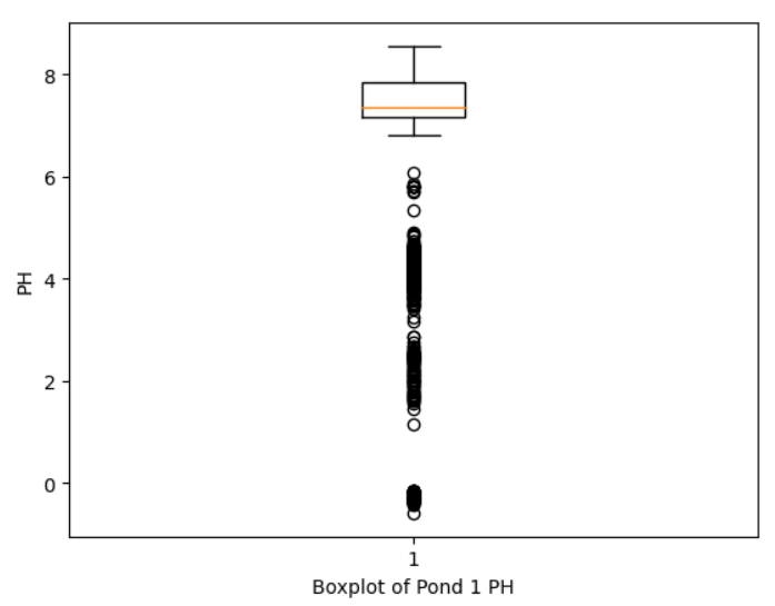
We note various issues with the statistics. The average levels of ammonia, nitrate, and dissolved oxygen are incredibly high. Ammonia is incredibly toxic to fish even at 1 mg/L. Ideally, we want ammonia to be 0 (see Chapter 3 of FAO). We suspect that the columns have been scaled in some way. Fortunately, the data transformation we perform later will remove this unknown scaling. In general, it’s not harmful to have high level of nitrate, but large amount of nitrate indicates inefficiency. We should add more yummy veggies. The average of pH is 7.5, which would lead to nutrient deficiencies. Plants absorb nutrients better under a slightly acidic environment, preferably between 6-7 (see Lennard and Goddek, 2019). We obtain the plot and boxplot of Pond 1’s pH below using

plt.boxplot(pond1.PH)
plt.ylabel('PH')
plt.xlabel('Boxplot of Pond 1 PH')

plt.plot(pond1.PH)
plt.xlabel('Time')
plt.ylabel('PH')
plt.title('Pond 1 PH')

The readings for pH were definitely incorrect at the end. Let’s look at the hourly data of Pond 1. By looking at hourly data, we should be able to remove outliers due to errors in the sensors.

From the plots above, we observe that the pH is becoming more neutral as the system is more established, which is preferable as mentioned above. Around t=50, the fish starts to grow quickly, which of course would lead to high nitrates from the nitrifying bacterias. However, the nitrate level is not decreasing, which means more vegetation were not added to utilize the nitrates. The ammonia level is relatively low for the most part, which means the high levels of ammonia we saw earlier were due to sensor error. (When we constructed the plots above, we thought the rows were at 5-second intervals. We will adjust this later in the series.)

In the next post, we will combine the data from six of the ponds together and sort by time. We then filter out the rows with astronomically large ammonia levels. This should still give us plenty of data while filtering bad data due to sensor errors.