Sophelen Research

PART 2: DATA TRANSFORMATION

This is a continuation of the post Basic deep learning with aquaponics, Part 1.

Recall that we are working with the aquaponics data from

https://www.kaggle.com/datasets/ogbuokiriblessing/sensor-based-aquaponics-fish-pond-datasets

In this post, we will combine the data from Pond 1 to Pond 4 and Pond 6 together, we will remove certain columns, and perform data transformations as mentioned in Part 1 so that we can have a better picture of the dataset overall. It would be nice to combine data from all ponds together, but there are many inconsistencies across the ponds. Combining the tables together would help us smooth out outliers due to sensor errors. A sizable portion of the dates will be duplicated, so we will replace the columns with their means. Furthermore, to be able to combine, we have to make sure that all the ponds start at the same date, if not, we have to adjust the date column. For example, Pond 12 starts a week later than the other ponds. Here, we can look at the heads and tails of the ponds:

ponds=[pond1,pond2,pond3,pond4,pond6]
for pond in ponds:
  print(pond.date.head())
  print(pond.date.tail())

Note that we are working with a time series, so we have to be especially careful. I am not a data scientist, so time series is always frightening to me. In the future, we will use RNN to create a model to detect anomaly in the pond. Here we are combining various tables together, so the date column becomes less meaningful. Later on, we may have to look at each individual pond to perform certain tasks.

For each pond, we will rename and choose only the columns date, temperature, dissolved oxygen, ammonia, nitrate, and weight. For Pond 1 to Pond 6, we perform the following

pond1=pd.read_csv('IoTPond1.csv')
pond1.dropna(inplace=True)
pond1.rename(columns={'created_at':'date', 'Temperature (C)':'temp', 'Dissolved Oxygen(g/ml)':'DO','Ammonia(g/ml)':'ammonia','Nitrate(g/ml)':'nitrate', 'Fish_Weight(g)':'weight'}, inplace=True)
pond1.drop(['entry_id','Turbidity(NTU)','Fish_Length(cm)','Population'], axis=1,inplace=True)
pond1.date=pd.to_datetime(pond1.date,dayfirst=False)

We then concatenate the five tables, sort by date, and choose only rows where ammonia is less 1000 and pH is greater than 0. If we do not exclude these values, the statistics on ammonia will go to infinity. Basically, the errors from one pond get filled by data from other ponds. I was going to include all 11 ponds, but I got tired.

data=pd.concat([pond1,pond2,pond3,pond4,pond6])
data.sort_values(by='date', inplace=True)
data=data[(data.ammonia < 1000) & (data.PH > 0)]
data.reset_index(drop=True, inplace=True)
median_values = data.groupby('date').transform('mean')
data.iloc[:, 1:] = median_values
data.drop_duplicates(subset='date', inplace=True)
data.describe()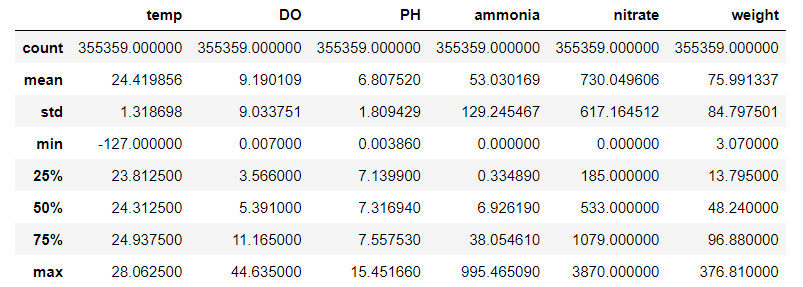

Our new data now has 355359 rows. Good thing we stop at Pond 6, else we may need PySpark to handle large data lol. Note that some of the statistics do not make sense. For example, the minimum temperature is -127 C. Perhaps now it’s a good idea to look at the heatmap of the correlation matrix to see how the various variables are correlated.

sns.heatmap(data=data.corr(), cmap='coolwarm', annot=True, linewidth=1)
plt.title('Correlation matrix')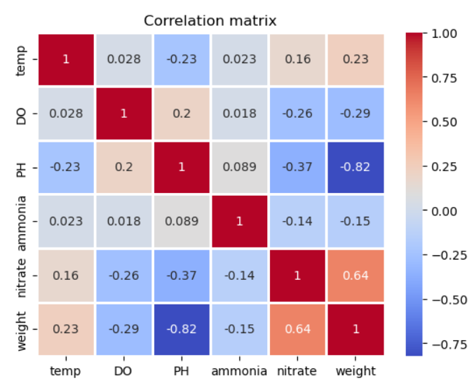

From the heatmap, we see that there is strong correlation between weight, nitrate, and ammonia, which is as expected. When the pH is high, the nitrifying bacterias can not convert ammonia to nitrates, so the correlation is negative. Furthermore, as the fish grows larger, there is more ammonia for the bacterias to convert to nitrates. When ammonia is oxidized into nitrites and nitrates, hydrogen ions are produced, thus decreasing the pH level. On the other hand, the temperature and dissolved oxygen levels are usually kept constant, so there is very little variance to have correlation with the weight. This tells us that we can remove dissolved oxygen and temperature from our model with negligible effect. Note that the correlation between pH and weight should not be that high as we generally keep the pH level balanced. Earlier, we saw that there were errors in the pH readings.

We will scale our combined data using the MixMaxScaler. Note that if we wish to use our data for any type of modeling, we must split our data first before doing any transformation to prevent data leakage. We will do this in Part 4.

We then define a processing function to make transformation more modular. Note we below that we use ColumnTransformer in case we have categorical columns for other types of data. Of course, the numbers no longer make sense, but they will help us understand the overall picture.

def preprocess(data):
num_features = data.select_dtypes(include=[‘float64’, ‘int64’])
num_cols = num_features.columns
ct=ColumnTransformer([(‘scale’, MinMaxScaler(), num_cols)], remainder=’passthrough’)
return pd.DataFrame(ct.fit_transform(data),columns=num_cols)
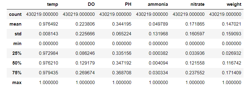
data_scaled = preprocess(data.iloc[:,1:],True)
data_scaled.describe()

Now, if we plot every 10,000th row, things look nicer.

columns=['PH', 'ammonia', 'nitrate', 'weight']
data_scaled['date']=data['date']
data_to_plot=data_scaled[data_scaled.index % 10000 == 0]
for column in columns:
  plt.plot(data_to_plot.date, data_to_plot[column],label=column)
plt.xticks(rotation=45)
plt.title('Scaled levels versus dates')
plt.legend()
plt.show()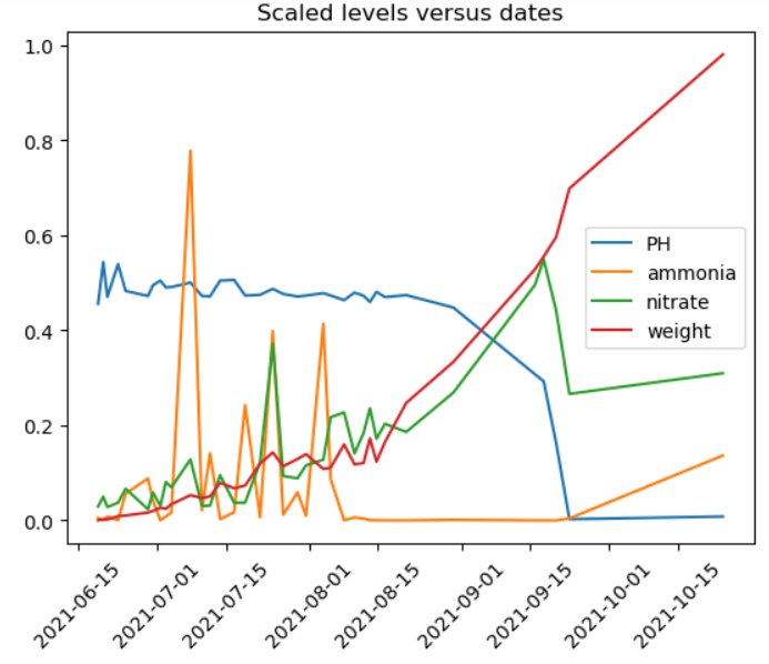

Note that even though ammonia level spiked a few times, eventually it stabilized. The nitrate level kept increasing, which indicates inefficiency. A large amount of nitrates were not utilized. Finally, we observe that the pH levels are not correct at the end, which cause the correlation between pH and weight to be very high as we noted above.

In the next post, we will discuss on the basics of aquaponics.

These are the libraries that we imported

import pandas as pd
import numpy as np
from matplotlib import pyplot as plt
import seaborn as sns
from sklearn.model_selection import train_test_split
from sklearn.compose import ColumnTransformer
from sklearn.preprocessing import MinMaxScaler
%matplotlib inline